import pandas as pd
import numpy as np
import matplotlib.pyplot as plt
import seaborn as sns
zoo = pd.read_csv("https://raw.githubusercontent.com/selva86/datasets/refs/heads/master/Zoo.csv")
Chapter # 08
Decision Tree for Classification & Regression
Chapter # 08
Decision Tree for Classification & Regression
Introduction
Decision Tree (DT) is a supervised Machine Learning (ML) algorithm; however, it is not an individual algorithm, rather it refers to a set of algorirthms that use decision tree structure. The DT can solve both classification and regression tasks, handle continuous and categorical predictors, and are suited to sloving multi-class classification problems. Decision tree forms a flow chart like structure that’s why they are very easy to interpret and understand. It is one of the few ML algorithms where it is very easy to visualize and analyze the internal working of algorithm. The decision tree is a distribution-free or non-parametric method, which does not depend upon probability distribution assumptions. Decision trees can handle high dimensional data with good accuracy. Moreover, Its training time is faster compared to the neural network algorithm. The time complexity of decision trees is a function of the number of records and number of attributes in the given data.
The basic premise of all tree-based classification algorithms is that they learn a sequence of questions that separates cases into different classes. Each question has a binary answer, and cases will be sent down the left or right branch depending on which criteria they meet. There can be branches within branches; and once the model is learned, it can be graphically represented as a tree.
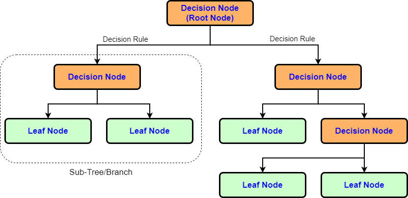
Just like flowchart, decision tree contains different types of nodes and branches. Figure 1 shows the basic structure of decision tree algorithm. Every decision node represent the test on feature and based on the test result it will either form another branch or the leaf node.
Decision Tree Algorithm Terminology
There are several terms in DT. Understanding of the those terms is important. Some of the terms are elaborated below -
Root Node- The question parts of the tree are called nodes, and the very first question/node is called the root node. Nodes have one branch leading to them and two branches leading away from themSplitting- It is a process of dividing a node into two or more sub-nodesDecision Node- When a sub-node splits into further sub-nodes, then it is called a decision nodeLeaf/Terminal Node- Nodes that do not split are called Leaf or Terminal nodes. Leaf nodes have a single branch leading to them but no branches leading away from themPruning- When we remove sub-nodes of a decision node, this process is called pruning. It is the opposite process of splittingBranch/Sub Tree- A sub-section of an entire tree is called a branch or sub-treeParent and Child Node- A node, which is divided into sub-nodes is called the parent node of sub-nodes where sub-nodes are the children of a parent node
How Does Decision Tree Work?
At each stage of the tree-building process, the decision tree algorithm considers all of the predictor variables and selects the predictor that does the best job of discriminating the classes. It starts at the root and then, at each branch, looks again for the next feature that will best discriminate the classes of the cases that took that branch.
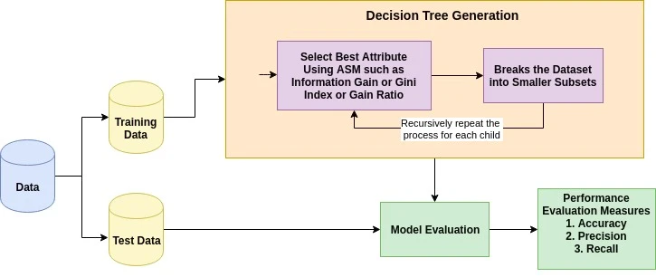
To sum up, the steps decision tree follows are given below. Figure 2 shows how decision tree works.
Select the best attribute using Attribute Selection Measures (ASM) to split the cases
Make that attribute a decision node and breaks the dataset into smaller subsets
Start tree builiding by repeating this process recursively for each child until one of the following conditions matches -
All the data points (or tuples) in a particular node of the tree have the same value for a specific attribute. This typically happens when the node is a leaf node, indicating that the data points have been perfectly classified according to the target attribute. In other words, there’s no further need to split the node because it already represents a homogeneous group with respect to the target attribute. For example, if you’re classifying animals and you reach a node where all the animals are “mammals,” then all the tuples in that node belong to the same attribute value “mammal.” This means the decision tree has successfully classified this subset of data.
There are no more remaining attributes
There are no more instances
Attribute Selection Measures (ASM)
The objective of decision tree is to split the data in such a way that at the end we have different groups of data which has more similarity (Homogeneousness) and less randomness/impurity1 (Heterogenousness). In order to achieve this, every split in decision tree must reduce the randomness. Decision tree uses entropy (Information Gain) or gini index (Gini Gain) selection criteria to split the categorical outcome variable (classification), but uses mse, friedman_mse and mae continuous outcome variable (regression).
Entropy (Information Gain)
In order to find the best feature which will reduce the randomness after a split, we can compare the randomness before and after the split for every feature. In the end we choose the feature which will provide the highest reduction in randomness. Formally randomness in data is known as Entropy and difference between the Entropy before and after split is known as Information Gain. Since decision trees will have multiple branches, information gain formula is -
\[Information Gain = Entropy (Parent Decision Node) - (Average Entropy (Child Nodes))\]
The formula for Entropy is -
\[Entropy = \sum_i - P_i log_2 P_i\]
Above, the subscript i indicates the classes in target variable.
Gini Index (Gini Gain)
In case of gini impurity, we pick a random data point in our dataset. Then randomly classify it according to the class distribution in the dataset. So it becomes very important to know the accuracy of this random classification. Gini impurity gives us the probability of incorrect classification. We’ll determine the quality of the split by weighting the impurity of each branch by how many elements it has. Resulting value is called as ‘Gini Gain’ or ‘Gini Index’. This is what’s used to pick the best split in a decision tree. The Higher the gini gain, the better the split.
\[ Gini = 1 - \sum_iP^2_i\]
Figure 3 shows gini index for a subtree (parent and child node) -
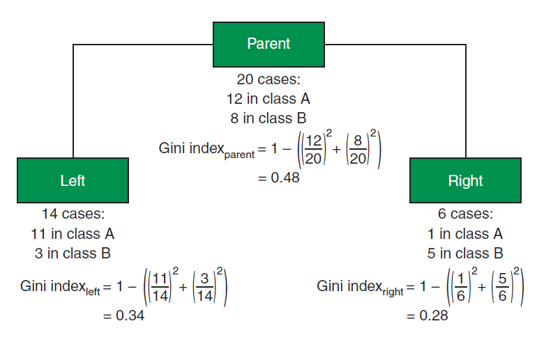
\[ Gini index_{split} = p(left)\times Gini Index_{left} + p(right)\times Gini index_{right}\] \[ Gini index_{split} = {14 \over 20}\times 0.34 + {6\over 20}\times 0.28 = 0.32\]
\[Gini Gain = 0.48 - 0.32 = 0.16\]
Hyperparameter in Decision Tree
Decision tree algorithms are described as greedy. By greedy, we mean they search for the split that will perform best at the current node, rather than the one that will produce the best result globally. For example, a particular split might discriminate the classes best at the current node but result in poor separation further down that branch. Conversely, a split that results in poor separation at the current node may yield better separation further down the tree. Decision tree algorithms would never pick this second split because they only look at locally optimal splits, instead of globally optimal ones. Therefore, there are three issues with the approach -
The algorithm isn’t guaranteed to learn a globally optimal model.
If left unchecked, the tree will continue to grow deeper until all the leaves are pure (of only one class).
For large datasets, growing extremely deep trees becomes computationally expensive.
Overfitting in Decision Tree Algorithm
While it’s true that decision tree algorithm isn’t guaranteed to learn a globally optimal model, the depth of the tree is of greater concern to us. Besides the computational cost, growing a full-depth tree until all the leaves are pure is very likely to overfit the training set and create a model with high variance. This is because as the feature space is split up into smaller and smaller pieces, we’re much more likely to start modeling the noise in the data.
How do we guard against such extravagant tree building? There are two ways of doing it:
Grow a full tree, and then prune it (Post-pruning)
Employ stopping criteria (Pre-pruning)
In the first approach, we allow the greedy algorithm to grow its full, overfit tree, and then we get out our garden shears and remove leaves that don’t meet certain criteria. This process is imaginatively named pruning, because we end up removing branches and leaves from our tree. This is sometimes called bottom-up pruning because we start from the leaves and prune up toward the root.
In the second approach, we include conditions during tree building that will force splitting to stop if certain criteria aren’t met. This is sometimes called top-down pruning because we are pruning the tree as it grows down from the root.
Both approaches may yield comparable results in practice, but there is a slight computational edge to top-down pruning because we don’t need to grow full trees and then prune them back. For this reason, we will use the stopping criteria approach.
The stopping criteria we can apply at each stage of the tree-building process are as follows:
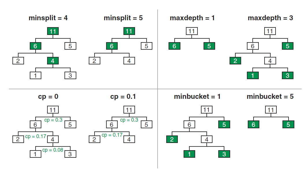
Minimum number of cases in a node before splitting (
min_samples_splitargument in scikit learn) - This parameter specifies the minimum number of samples required to split an internal node. By setting this parameter, you can control the minimum number of cases (or samples) that must be present in a node before it can be split into smaller nodes.Maximum depth of the tree (
max_depth) - This parameter controls the maximum number of levels in the tree. By setting this parameter, you can limit the depth of the tree to prevent overfitting.Minimum improvement in performance for a split (
min_impurity_decrease) - This parameter specifies the minimum decrease in impurity required for a node to be split. By setting this parameter, you can control the minimum improvement in performance needed to justify a split.Minimum number of cases in a leaf (
min_samples_leaf) - This parameter specifies the minimum number of samples required to be at a leaf node. By setting this parameter, you can control the minimum number of cases (or samples) that must be present in a leaf node.
Figure 4 shows some of these stopping criteria -
Pros and Cons of Decision Tree Algorithm
There are many advantages of using decision tree. However, it also involves some cons. Some pros and cons are discussed below -
Advantages -
Simple to understand and to interpret. Trees can be visualized.
Requires little data preparation. Other techniques often require data normalization, dummy variables need to be created and blank values to be removed. Note however that this algorithm does not support missing values.
Able to handle both numerical and categorical data.
Able to handle multi-output problems.
Uses a white box model. Results are easy to interpret.
Possible to validate a model using statistical tests. That makes it possible to account for the reliability of the model.
The decision tree has no assumptions about distribution because of the non-parametric nature of the algorithm.
It can be used for feature engineering such as predicting missing values, suitable for variable selection.
It can easily capture Non-linear patterns.
Disadvantages -
Decision-tree learners can create over-complex trees that do not generalize the data well. This is called overfitting. Mechanisms such as pruning, setting the minimum number of samples required at a leaf node or setting the maximum depth of the tree are necessary to avoid this problem.
Decision trees can be unstable because small variations in the data might result in a completely different tree being generated. This problem is mitigated by using decision trees within an ensemble.
Decision tree learners create biased trees if some classes dominate. It is therefore recommended to balance the dataset prior to fitting with the decision tree.
Building Decision Tree Model in scikit learn
zoo.info()<class 'pandas.core.frame.DataFrame'>
RangeIndex: 101 entries, 0 to 100
Data columns (total 17 columns):
# Column Non-Null Count Dtype
--- ------ -------------- -----
0 hair 101 non-null bool
1 feathers 101 non-null bool
2 eggs 101 non-null bool
3 milk 101 non-null bool
4 airborne 101 non-null bool
5 aquatic 101 non-null bool
6 predator 101 non-null bool
7 toothed 101 non-null bool
8 backbone 101 non-null bool
9 breathes 101 non-null bool
10 venomous 101 non-null bool
11 fins 101 non-null bool
12 legs 101 non-null int64
13 tail 101 non-null bool
14 domestic 101 non-null bool
15 catsize 101 non-null bool
16 type 101 non-null object
dtypes: bool(15), int64(1), object(1)
memory usage: 3.2+ KBzoo.isna().sum()hair 0
feathers 0
eggs 0
milk 0
airborne 0
aquatic 0
predator 0
toothed 0
backbone 0
breathes 0
venomous 0
fins 0
legs 0
tail 0
domestic 0
catsize 0
type 0
dtype: int64import sklearn # Declare feature vector and target variable
X = zoo.drop(columns = ['type'], axis = 1)
y = zoo['type'] # Split Data into Training and Testing
from sklearn.model_selection import train_test_split
X_train, X_test, y_train, y_test = train_test_split(X,y, test_size = 0.20,
random_state = 2025)Decision Tree using gini
from sklearn.tree import DecisionTreeClassifier
from sklearn.metrics import accuracy_score, confusion_matrix
#####################################
# Decision Tree using Gini Index
#####################################

tree_gini = DecisionTreeClassifier(criterion = "gini")
tree_gini.fit(X_train, y_train)

y_pred = tree_gini.predict(X_test)

accuracy = accuracy_score(y_test, y_pred)
print(f"Accuracy: {accuracy}")
Accuracy: 0.9047619047619048# Plotting Decision Tree
plt.figure(figsize=(12,8))
from sklearn import tree
tree.plot_tree(tree_gini.fit(X_train, y_train))[Text(0.7777777777777778, 0.9285714285714286, 'x[3] <= 0.5\ngini = 0.767\nsamples = 80\nvalue = [3, 14, 11, 8, 32, 8, 4]'),
Text(0.6666666666666666, 0.7857142857142857, 'x[1] <= 0.5\ngini = 0.796\nsamples = 48\nvalue = [3, 14, 11, 8, 0, 8, 4]'),
Text(0.7222222222222222, 0.8571428571428572, 'True '),
Text(0.5555555555555556, 0.6428571428571429, 'x[11] <= 0.5\ngini = 0.763\nsamples = 34\nvalue = [3, 0, 11, 8, 0, 8, 4]'),
Text(0.4444444444444444, 0.5, 'x[7] <= 0.5\ngini = 0.711\nsamples = 23\nvalue = [3, 0, 0, 8, 0, 8, 4]'),
Text(0.2222222222222222, 0.35714285714285715, 'x[9] <= 0.5\ngini = 0.5\nsamples = 16\nvalue = [0, 0, 0, 8, 0, 8, 0]'),
Text(0.1111111111111111, 0.21428571428571427, 'gini = 0.0\nsamples = 6\nvalue = [0, 0, 0, 0, 0, 6, 0]'),
Text(0.3333333333333333, 0.21428571428571427, 'x[12] <= 3.0\ngini = 0.32\nsamples = 10\nvalue = [0, 0, 0, 8, 0, 2, 0]'),
Text(0.2222222222222222, 0.07142857142857142, 'gini = 0.0\nsamples = 2\nvalue = [0, 0, 0, 0, 0, 2, 0]'),
Text(0.4444444444444444, 0.07142857142857142, 'gini = 0.0\nsamples = 8\nvalue = [0, 0, 0, 8, 0, 0, 0]'),
Text(0.6666666666666666, 0.35714285714285715, 'x[5] <= 0.5\ngini = 0.49\nsamples = 7\nvalue = [3, 0, 0, 0, 0, 0, 4]'),
Text(0.5555555555555556, 0.21428571428571427, 'gini = 0.0\nsamples = 3\nvalue = [0, 0, 0, 0, 0, 0, 3]'),
Text(0.7777777777777778, 0.21428571428571427, 'x[9] <= 0.5\ngini = 0.375\nsamples = 4\nvalue = [3, 0, 0, 0, 0, 0, 1]'),
Text(0.6666666666666666, 0.07142857142857142, 'gini = 0.0\nsamples = 1\nvalue = [0, 0, 0, 0, 0, 0, 1]'),
Text(0.8888888888888888, 0.07142857142857142, 'gini = 0.0\nsamples = 3\nvalue = [3, 0, 0, 0, 0, 0, 0]'),
Text(0.6666666666666666, 0.5, 'gini = 0.0\nsamples = 11\nvalue = [0, 0, 11, 0, 0, 0, 0]'),
Text(0.7777777777777778, 0.6428571428571429, 'gini = 0.0\nsamples = 14\nvalue = [0, 14, 0, 0, 0, 0, 0]'),
Text(0.8888888888888888, 0.7857142857142857, 'gini = 0.0\nsamples = 32\nvalue = [0, 0, 0, 0, 32, 0, 0]'),
Text(0.8333333333333333, 0.8571428571428572, ' False')]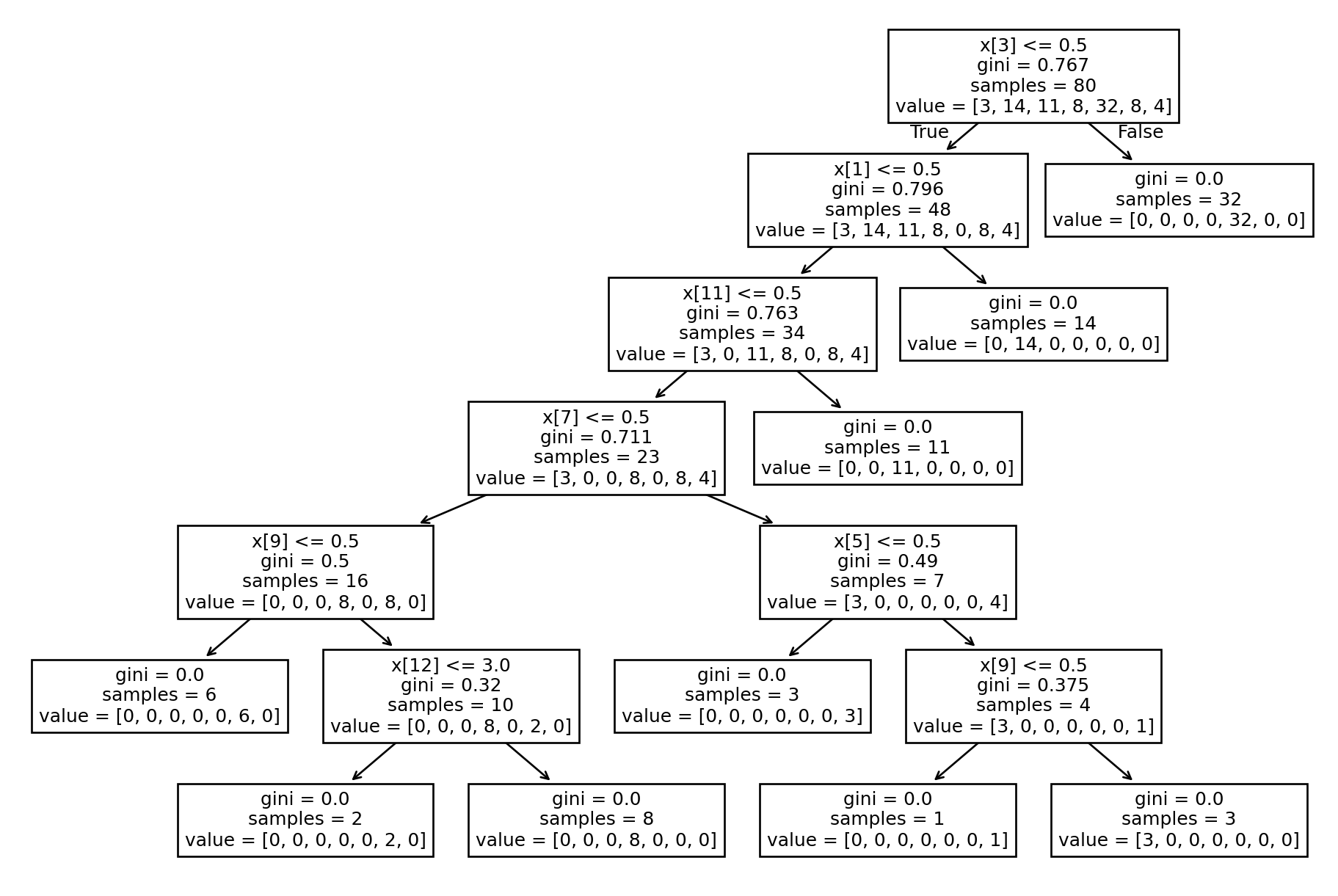
# Compare Train and Test set Accuracy
y_pred_train_gini = tree_gini.predict(X_train)
print('Training-set accuracy score: {0:0.4f}'. format(accuracy_score(y_train, y_pred_train_gini)))

# Check for overfitting and underfitting
print('Training set score: {:.4f}'.format(tree_gini.score(X_train, y_train)))
print('Test set score: {:.4f}'.format(tree_gini.score(X_test, y_test)))
Training-set accuracy score: 1.0000
Training set score: 1.0000
Test set score: 0.9048Decision Tree using entropy
#####################################
# Decision Tree using entropy (Information Gain)
#####################################
tree_entropy = DecisionTreeClassifier(criterion = "entropy")

tree_entropy.fit(X_train, y_train)

y_pred = tree_entropy.predict(X_test)

accuracy = accuracy_score(y_test, y_pred)
print(f"Accuracy: {accuracy}")
Accuracy: 0.8571428571428571# Plotting Decision Tree
plt.figure(figsize=(12,8))
tree.plot_tree(tree_entropy.fit(X_train, y_train))[Text(0.6666666666666666, 0.9166666666666666, 'x[3] <= 0.5\nentropy = 2.421\nsamples = 80\nvalue = [3, 14, 11, 8, 32, 8, 4]'),
Text(0.5555555555555556, 0.75, 'x[7] <= 0.5\nentropy = 2.416\nsamples = 48\nvalue = [3, 14, 11, 8, 0, 8, 4]'),
Text(0.6111111111111112, 0.8333333333333333, 'True '),
Text(0.3333333333333333, 0.5833333333333334, 'x[8] <= 0.5\nentropy = 1.53\nsamples = 30\nvalue = [0, 14, 0, 8, 0, 8, 0]'),
Text(0.2222222222222222, 0.4166666666666667, 'x[9] <= 0.5\nentropy = 1.0\nsamples = 16\nvalue = [0, 0, 0, 8, 0, 8, 0]'),
Text(0.1111111111111111, 0.25, 'entropy = 0.0\nsamples = 6\nvalue = [0, 0, 0, 0, 0, 6, 0]'),
Text(0.3333333333333333, 0.25, 'x[12] <= 3.0\nentropy = 0.722\nsamples = 10\nvalue = [0, 0, 0, 8, 0, 2, 0]'),
Text(0.2222222222222222, 0.08333333333333333, 'entropy = 0.0\nsamples = 2\nvalue = [0, 0, 0, 0, 0, 2, 0]'),
Text(0.4444444444444444, 0.08333333333333333, 'entropy = 0.0\nsamples = 8\nvalue = [0, 0, 0, 8, 0, 0, 0]'),
Text(0.4444444444444444, 0.4166666666666667, 'entropy = 0.0\nsamples = 14\nvalue = [0, 14, 0, 0, 0, 0, 0]'),
Text(0.7777777777777778, 0.5833333333333334, 'x[11] <= 0.5\nentropy = 1.347\nsamples = 18\nvalue = [3, 0, 11, 0, 0, 0, 4]'),
Text(0.6666666666666666, 0.4166666666666667, 'x[12] <= 2.0\nentropy = 0.985\nsamples = 7\nvalue = [3, 0, 0, 0, 0, 0, 4]'),
Text(0.5555555555555556, 0.25, 'entropy = 0.0\nsamples = 3\nvalue = [0, 0, 0, 0, 0, 0, 3]'),
Text(0.7777777777777778, 0.25, 'x[5] <= 0.5\nentropy = 0.811\nsamples = 4\nvalue = [3, 0, 0, 0, 0, 0, 1]'),
Text(0.6666666666666666, 0.08333333333333333, 'entropy = 0.0\nsamples = 1\nvalue = [0, 0, 0, 0, 0, 0, 1]'),
Text(0.8888888888888888, 0.08333333333333333, 'entropy = 0.0\nsamples = 3\nvalue = [3, 0, 0, 0, 0, 0, 0]'),
Text(0.8888888888888888, 0.4166666666666667, 'entropy = 0.0\nsamples = 11\nvalue = [0, 0, 11, 0, 0, 0, 0]'),
Text(0.7777777777777778, 0.75, 'entropy = 0.0\nsamples = 32\nvalue = [0, 0, 0, 0, 32, 0, 0]'),
Text(0.7222222222222222, 0.8333333333333333, ' False')]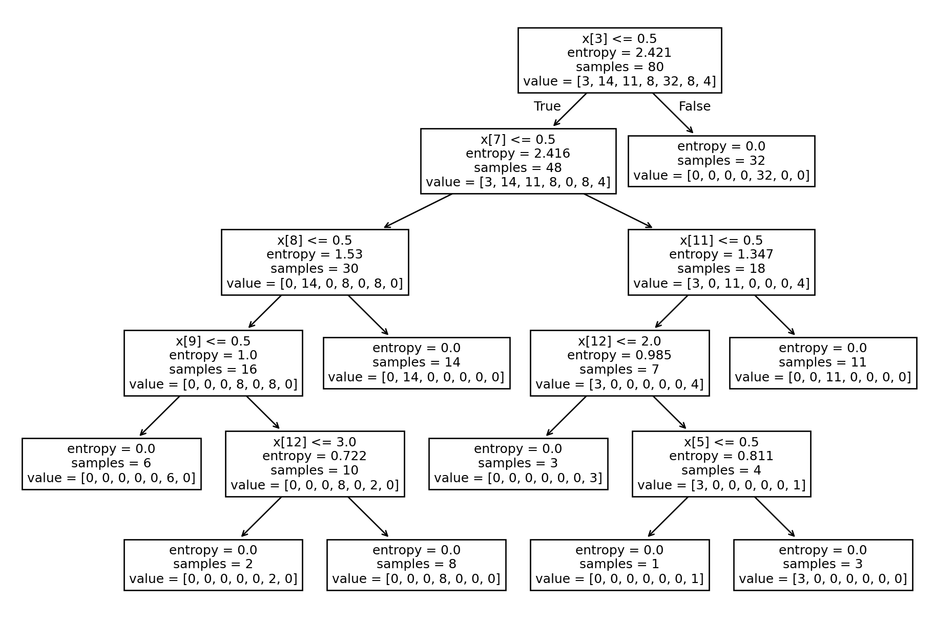
# Compare Train and Test set Accuracy
y_pred_train_entropy = tree_entropy.predict(X_train)
print('Training-set accuracy score: {0:0.4f}'. format(accuracy_score(y_train, y_pred_train_entropy)))

# Check for overfitting and underfitting
print('Training set score: {:.4f}'.format(tree_entropy.score(X_train, y_train)))
print('Test set score: {:.4f}'.format(tree_entropy.score(X_test, y_test)))
Training-set accuracy score: 1.0000
Training set score: 1.0000
Test set score: 0.9048Hyperparameter Tuning with Cross Validation
####################################################
# Hyperparameter Tuning
####################################################
from sklearn.model_selection import GridSearchCV, StratifiedKFold

tree_hyp = DecisionTreeClassifier(random_state=420)
tree_hyp.fit(X_train, y_train)
param = {
    'min_samples_split': np.arange(5,21),
    'min_samples_leaf': np.arange(3,11),
    'max_depth': np.arange(3,11),
    'ccp_alpha': np.arange (0.01, 0.10)

}

Kfold = StratifiedKFold(n_splits=5, shuffle=True, random_state=19)
# Creating the grid
best = GridSearchCV(estimator = tree_hyp,param_grid=param, cv = Kfold, n_jobs = -1, verbose = 1)
best.fit(X_train, y_train)
best.best_params_ # Best set of parameters Fitting 5 folds for each of 1024 candidates, totalling 5120 fitsc:\Users\mshar\OneDrive - Southern Illinois University\BSAN405_MLINBUSINESS_WEBSITE\mlbusiness2\Lib\site-packages\sklearn\model_selection\_split.py:805: UserWarning: The least populated class in y has only 3 members, which is less than n_splits=5.
warnings.warn({'ccp_alpha': np.float64(0.01),
'max_depth': np.int64(6),
'min_samples_leaf': np.int64(3),
'min_samples_split': np.int64(5)}best.best_estimator_ # best estimatorDecisionTreeClassifier(ccp_alpha=np.float64(0.01), max_depth=np.int64(6),
min_samples_leaf=np.int64(3),
min_samples_split=np.int64(5), random_state=420)In a Jupyter environment, please rerun this cell to show the HTML representation or trust the notebook. On GitHub, the HTML representation is unable to render, please try loading this page with nbviewer.org.
DecisionTreeClassifier(ccp_alpha=np.float64(0.01), max_depth=np.int64(6),
                       min_samples_leaf=np.int64(3),
min_samples_split=np.int64(5), random_state=420)y_pred_hyp = best.predict(X_test)
accuracy_score(y_pred_hyp, y_test)0.9523809523809523pd.DataFrame(best.cv_results_).head()| mean_fit_time | std_fit_time | mean_score_time | std_score_time | param_ccp_alpha | param_max_depth | param_min_samples_leaf | param_min_samples_split | params | split0_test_score | split1_test_score | split2_test_score | split3_test_score | split4_test_score | mean_test_score | std_test_score | rank_test_score | |
|---|---|---|---|---|---|---|---|---|---|---|---|---|---|---|---|---|---|
| 0 | 0.004857 | 0.000476 | 0.002548 | 0.000225 | 0.01 | 3 | 3 | 5 | {'ccp_alpha': 0.01, 'max_depth': 3, 'min_sampl... | 0.8125 | 0.875 | 0.75 | 0.75 | 0.75 | 0.7875 | 0.05 | 715 |
| 1 | 0.004898 | 0.001681 | 0.003669 | 0.002014 | 0.01 | 3 | 3 | 6 | {'ccp_alpha': 0.01, 'max_depth': 3, 'min_sampl... | 0.8125 | 0.875 | 0.75 | 0.75 | 0.75 | 0.7875 | 0.05 | 715 |
| 2 | 0.003391 | 0.000171 | 0.002193 | 0.000296 | 0.01 | 3 | 3 | 7 | {'ccp_alpha': 0.01, 'max_depth': 3, 'min_sampl... | 0.8125 | 0.875 | 0.75 | 0.75 | 0.75 | 0.7875 | 0.05 | 715 |
| 3 | 0.003478 | 0.000256 | 0.002116 | 0.000108 | 0.01 | 3 | 3 | 8 | {'ccp_alpha': 0.01, 'max_depth': 3, 'min_sampl... | 0.8125 | 0.875 | 0.75 | 0.75 | 0.75 | 0.7875 | 0.05 | 715 |
| 4 | 0.003655 | 0.000213 | 0.003082 | 0.001211 | 0.01 | 3 | 3 | 9 | {'ccp_alpha': 0.01, 'max_depth': 3, 'min_sampl... | 0.8125 | 0.875 | 0.75 | 0.75 | 0.75 | 0.7875 | 0.05 | 715 |
## Running the model using best hyperparameter
tree_best = best.best_estimator_
# predicting using the hyperparameter
accuracy_score(y_train,tree_best.predict(X_train))0.9625# confusion matrix
confusion_matrix (y_train, tree_best.predict(X_train))array([[ 3, 0, 0, 0, 0, 0, 0],
[ 0, 14, 0, 0, 0, 0, 0],
[ 0, 0, 11, 0, 0, 0, 0],
[ 0, 0, 0, 8, 0, 0, 0],
[ 0, 0, 0, 0, 32, 0, 0],
[ 0, 0, 0, 2, 0, 6, 0],
[ 1, 0, 0, 0, 0, 0, 3]])Conclusion
Footnotes
Impurity is a measure of how heterogenous the classes are within a node. Entropy and gini index are two ways of measuring impurity↩︎